The latest version of this document is now in our Github repository here. See that, not this…
This paper is a log of a RepRap Ltd ongoing research project to create a completely new type of 3D printer invented by Adrian Bowyer (to whom “I” below refers…).
(As with our other documentation, clicking on an image should bring up a larger version.)
The Initial Invention (25 July 2019)
The invention combines three ideas to make a fourth. The three are:
- The reverse-CT scan 3D printing technique from Berkeley and Lawrence Livermore,
- The open-source electric 3D scanning technique for 3D reconstruction from Spectra, and
- Electropolymerisation.
My overall synthesis of the three is to use an electric current to make a liquid plastic monomer polymerise to a solid in such a way that it forms a 3-dimensional object with a specified shape, and to do that with a single scan in a time of (I hope…) a few seconds. Let me start by describing the three precursor technologies in more detail:
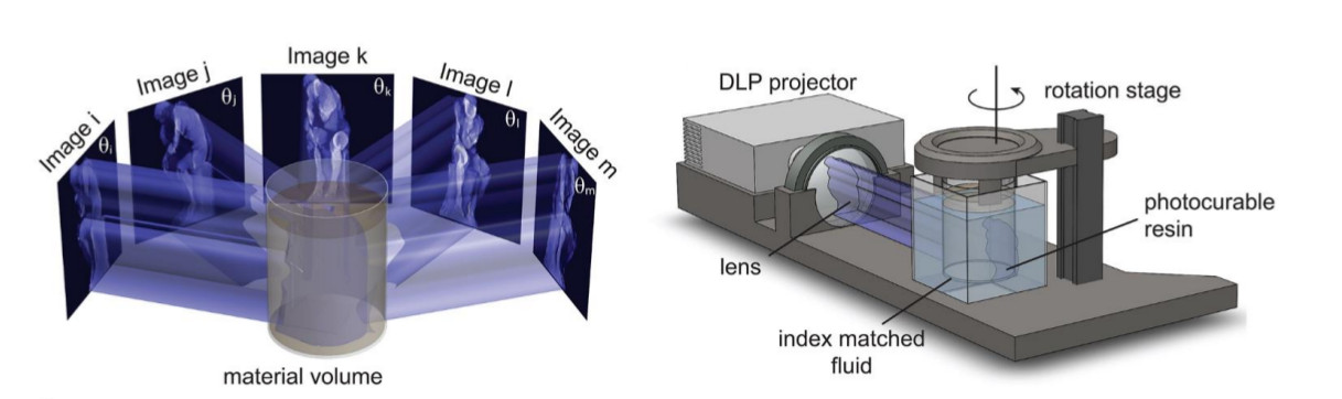
The Berkeley/Livermore system [thanks to B. E. Kelly et al., Science 10.1126/science.aau7114 (2019)].
Firstly, the Berkeley/Livermore system. What they do is to shine a light pattern from a digital projector into a bath of liquid monomer that contains a photoinitiator. Where a sufficient intensity of light falls, the monomer polymerises to form a solid. So far this description is like a conventional low-cost SLA system; but the really clever bit is that they treat the 3D object to be printed as if it were a CT scan. The light field is modulated in intensity as if it were (for example) X-rays passing through a patient on a scanner, and they rotate the scan so that a complete solid is formed in a single rotation in a matter of seconds. Computing the CT-scanner Radon Transform of a 3D-printing STL file is mathematically and computationally straightforward (it’s essentially just like ray-tracing for computer graphics). Neatly, their system does not need allowances to be made for refraction as the light enters the transparent rotating cylindrical bath containing the liquid monomer, because they submerge that in another bath that is rectangular, and so has flat faces for the light to pass through.

A preliminary scan of lung cross-section by the Spectra system [thanks to the Spectra Crowdfunder page].
Secondly, the Spectra system. This is an alternative way of CT scanning that does not use X-rays, but instead uses electric current. What they do is to place the object to be scanned in a bath of conducting liquid, and then apply a voltage from two small point-like electrodes on opposite sides of it and measure the current. The current takes multiple paths through the liquid around and through the object to be scanned, of course. But they then rotate the electrodes and repeat the measurement from a slightly different direction, just like rotating the X-ray source and the opposite detector in a conventional CT scanner. By repeatedly doing this they can gather enough information to construct a cross section of the object being scanned. By moving the electrodes at right angles to the cross section by a fraction of a millimetre and repeating the process they can make a stack of scans to digitise the scanned object as a full 3D solid. In practice more than two electrodes are used, and the current is switched electronically between them; this reduces mechanical complexity and increases speed.
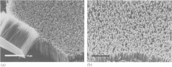
Nanowires made on a surface by electropolymerisation; scale bar is 10 μm [thanks to the Science Direct article on electropolymerisation].
Thirdly, Electropolymerisation. The clue here is in the name – this is causing a liquid monomer to polymerise to a solid by passing electricity through it rather than light (or other forms of energy).
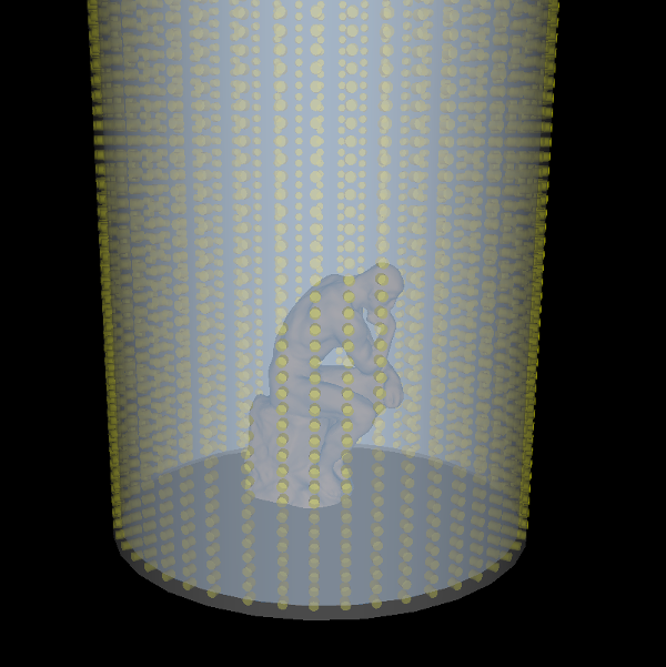
The Electric 3D Printing system proposed here.
I hope you can now see how these three concepts could work together. My idea is to have a bath of monomer engineered to polymerise using an electric current. In place of shining light through it like the Berkeley/Livermore system, the current is programmed using the reverse of the Spectra system. In its final form (shown in the diagram above), one would have a cylindrical bath containing the liquid monomer. The walls of the bath would have a fine array of electrodes in a square grid over their entire area (the grid would be finer than in the diagram). These would be addressed by a controlling computer to pass electric currents through the liquid monomer in such a way as to solidify it just where required to form the 3D solid defined by an STL file (as in conventional 3D printing). The machine would have no moving parts, and the solid would be formed in (I hope) a few seconds.
The entire machine could, of course, be printed in a conventional two-filament RepRap if one filament were conducting.
The primary purpose of the blog post of which this is a copy is to get my Electric 3D Printing idea out as open-source, and to establish it as prior art so that it cannot be patented.
Finally, and very speculatively, an even more ambitious possibility would be to move from organic chemistry to inorganic, and to replace the bath of monomer with an electrolyte such as copper acetate or copper sulphate. It might then be possible to cause the copper to precipitate at any location in 3D space if the pattern of electric currents through the liquid could be got right. The dense copper would settle out of solution, of course, so the process would have to start at the bottom of the bath and work up. I think that this idea would be much more difficult to make work than the polymerisation one. The reason is that I expect that the polymerisation system would turn out to rely on engineering a non-linear response in the polymerisation reaction to current: probably something like a sigmoid function. That would be very difficult (or even impossible) to do with metal deposition, which is a strictly linear Avogadro’s-number-and-coulombs phenomenon like electro-plating.
But if it could be made to work, we could then 3D-print a complete solid copper object at room temperature. Or, for that matter, a titanium one…
2 Dimensional Simulation (1 August 2019)
TL;DR: The simulation below works and gives sensible predictions. It has thrown up a problem that needs to be solved.
To try this out I decided to start by simulating it, which is to say I’ve written a mathematical model of the process to see if it’s possible to print shapes electrically in theory before going to the trouble of building an actual machine. The model has (unsurprisingly) some simplifying assumptions:
- Start with a 2D disc in the [x, y] plane, not a 3D volume in [x, y, z], and so see what happens for a single ring of electrodes that form a slice through the cylinder.
- Assume the conductivity of the liquid monomer doesn’t change when it sets solid.
- Assume that whether a node sets solid or not is decided by the total charge that moved through it for the entire process.
The model does not start with a shape that is to be printed and try to work out the pattern of voltage changes that would need to be made to create that shape. This would have to be done for the actual machine, but – before doing that – I decided just to apply patterns of voltages that seem as if they might make something sensible (like a cylinder in the middle) and see what they would actually do. This is much simpler than doing the backward calculation from the final desired shape.
Let V be the potentials over the disc, and E be the field. Then Laplace’s simplification of Poisson’s equation
$$\nabla^{2} V = 0,$$
when solved gives V, and E can then be found from
$$E = -\nabla V.$$
The current through any node will be proportional to the magnitude of the vector E at that node. Integrate that current over the time of the whole simulation, and you have the total charge that has run through that node, which should decide if it sets solid or not.
I wrote a finite-difference C++ program to solve for V over a disc. You can get the code from Github here; please let me know of any bugs you find. The obvious thing to do with a disc is to use the polar form of Laplace’s equation as the basis of the solution. But the problem with that is that angular resolution decreases with increasing radius unless you insert extra nodes, which makes things complicated. So I decided to use a rectangular Cartesian grid instead, and to code the disc in the boundary conditions.
In their simplest form those boundary conditions consist of a circular perimeter perpendicular to which the gradient vector, E, is forced to be 0 (which is to say that no current flows through the walls). Added to that are a couple of point electrodes diametrically opposite each other, one of which is at a positive voltage, and the other is negative. At these current does flow. Here is the solution for V over the disc for that situation on a 50×50 grid of nodes:
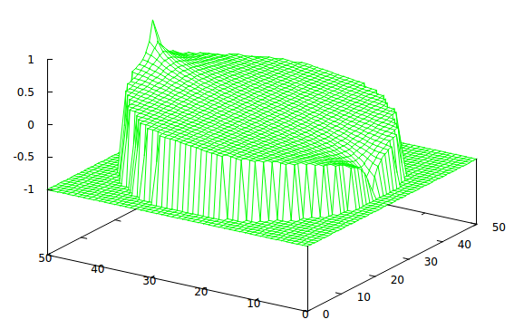
Potential, V, over the disc
The numbers don’t mean much – the picture would look the same but for scaling with 100 volts as with 1 volt. The flat area is outside the disc and can be ignored. The peak and the valley are the positive and negative electrodes, and the rest of the grid is the potential everywhere else. Taking the partial derivatives of V at each node with respect to x and y gives the vector E at that node. Pythagoras then gives the magnitude of E:
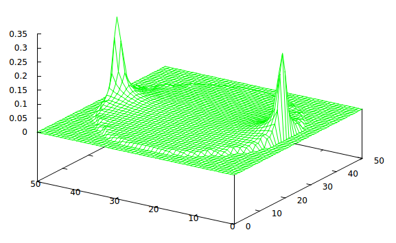
Field magnitude, |E|, over the disc.
As mentioned above, the current flowing through each node will be proportional to the value of the magnitude of E at the node. The currents are, as would be expected, greatest at the electrodes. But I was encouraged by the slope in the middle of the plot of the potentials, which corresponds to the non-zero plateau in the middle of the field magnitude plot. I thought that if one were to pass a series of currents from the electrodes as they were energised round the circle the sum of charges in the middle might exceed that at the individual electrodes, and so one would have built a solid disc in the middle and left liquid monomer round the outsides. Unfortunately, this did not happen. Here is the result of energising twenty pairs of electrodes in sequence and integrating the currents flowing through all the nodes for each one:
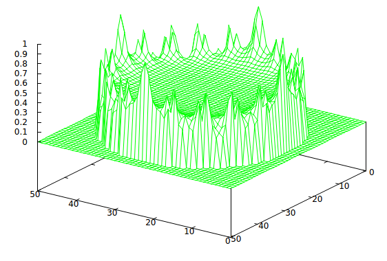
Integral of the current from twenty electrodes energised sequentially round the disc.
The jagged periphery is an aliasing effect from the grid, and doesn’t matter at this stage. As you can see there is a substantial charge plateau in the middle, but unfortunately it is still exceeded by the sums of the currents at the electrodes, even though 18 of them will be switched off for each individual energising. This means that the machine would tend to get clogged solid at the electrodes, regardless of what was going on in the middle.
This is discouraging. But it is only the simplest possible simulation of the simplest possible pattern of currents. There are many variables that I have not altered, such as different voltages at different electrodes (they don’t all have to be either off or on), different persistence times for one pattern, V, and fading dynamically between voltage patterns at the electrodes. Now I have the basic simulation written all these will be easy to experiment with.
If these experiments can be made to produce more hopeful results, then I will change the simulation to full 3D rather than the 2D disc. This is straightforward as it just means adding a z term to the partial differential equation along the cylinder axis and then solving in the entire cylindrical volume, rather than just a disc slice of it. Visualising the results will be rather like visualising a CT scan – a solid contour in the volume of constant charge integral would be triangulated and plotted in 3D.
2 Dimensional Simulation of Actual Printing (10 August 2019)
TL;DR: The simulation now “prints” simple shapes.
Obviously (after two days of thought…) if the machine prints solid where you don’t want, and doesn’t print where you do want, then all that is needed is to invert the process. In other words we need a polymer in which polymerisation is inhibited or reversed by electricity.
Remember Loctite:
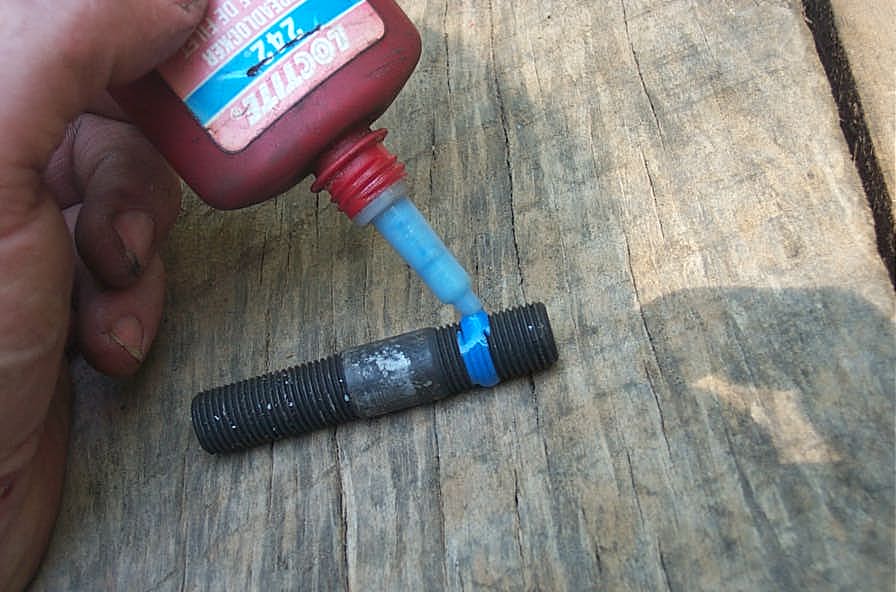
This is a remarkable material that polymerises solid except in the presence of oxygen, which keeps it monomeric. Thus when you tighten a nut and bolt with liquid Loctite on the threads this excludes the oxygen, solidifies the Loctite, and locks the nut to the bolt. Loosen them a bit to allow the oxygen back in, and the polymer depolymerises back to a liquid, and the threads can be undone easily because the reaction is also reversible. (The – possibly apocryphal – story is that Vernon Krieble, the inventor of Loctite, had greater difficulty making a bottle that would allow oxygen to permeate in to keep the stuff liquid than he did making Loctite itself.)
Let’s suppose that we can make a monomer that behaves like Loctite, but in which electricity takes the place of oxygen. Pass a current through it and it liquefies; turn it off and it solidifies. This would be useful stuff in its own right, but it would also be an ideal material for the electric 3D printing idea here.
The transition from solid to liquid with charge integral would not be instant. For this simulation I propose a sigmoid function, as I mentioned above:
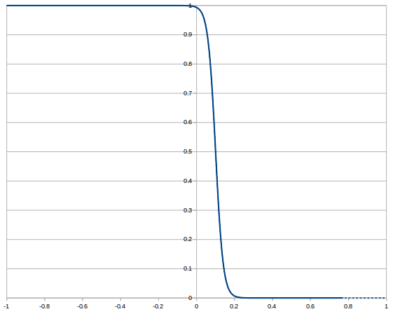
$$f(x) = 1 – e^{a(x – b)}/(e^{a(x – b)} + 1)$$
Ignore the negative bit of the abscissa; that’s just there for me to check things are correct; you can’t have negative charge integral just as you can’t have -3 apples. The variables a and b alter the shape and offset to the right of the sigmoid function and can be played around with in the simulation to experiment, or maybe one day to match the characteristics of a real polymer. The charge integral (the last surface plot above) was normalised to lie in the range [0, 1]. That is the value of x in the sigmoid function. The vertical axis is degree of polymerisation: 0 charge gives solid, and the (at the moment hypothetical) material liquifies as charge integral increases to the right, going fully liquid at a value around 0.2. Note at this stage these numbers aren’t real coulombs; they would be, however, proportional to real coulombs in a real machine. (The values a = 50 and b = 0.1 were used for this, incidentally.)
As with the last surface plot above, if we put 1 “volt” on each electrode round the circle in turn, along with -1 “volt” on the diametrically opposite electrode, we now print this:
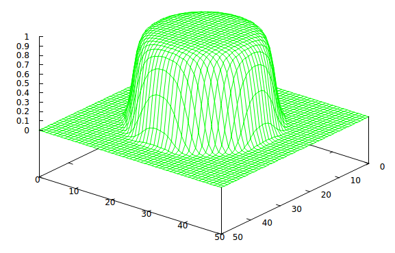
It’s solid in a circle in the middle, and liquid all around. We’ve printed a disc! Remember that the height of the surface from 0 to 1 represents the degree of polymerisation of the monomer – higher means more solid.
Now here’s what happens if we just put 1 “volt” on a quarter of the electrodes adjacent to each other and -1 “volt” on those diametrically opposite them:
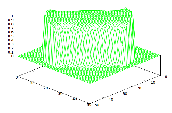
We’ve printed a (roughly) rectangular block.
I think it’s time to move the simulation from a 2D disc slice through the machine to a 3D cylinder that represents the entire machine.
3 Dimensional Simulation (13 August 2019)
The simulator now solves for Laplace’s equation in 3D.
Here’s the result of running round the bottom of the cylindrical reaction vessel in a circle putting 1 “volt” on each electrode and -1 “volt” on the opposite one, and moving up one level in Z then repeating that for the next ring of electrodes all the way up to the top. The transparent cylinder is the reaction vessel itself (without the electrodes for clarity):
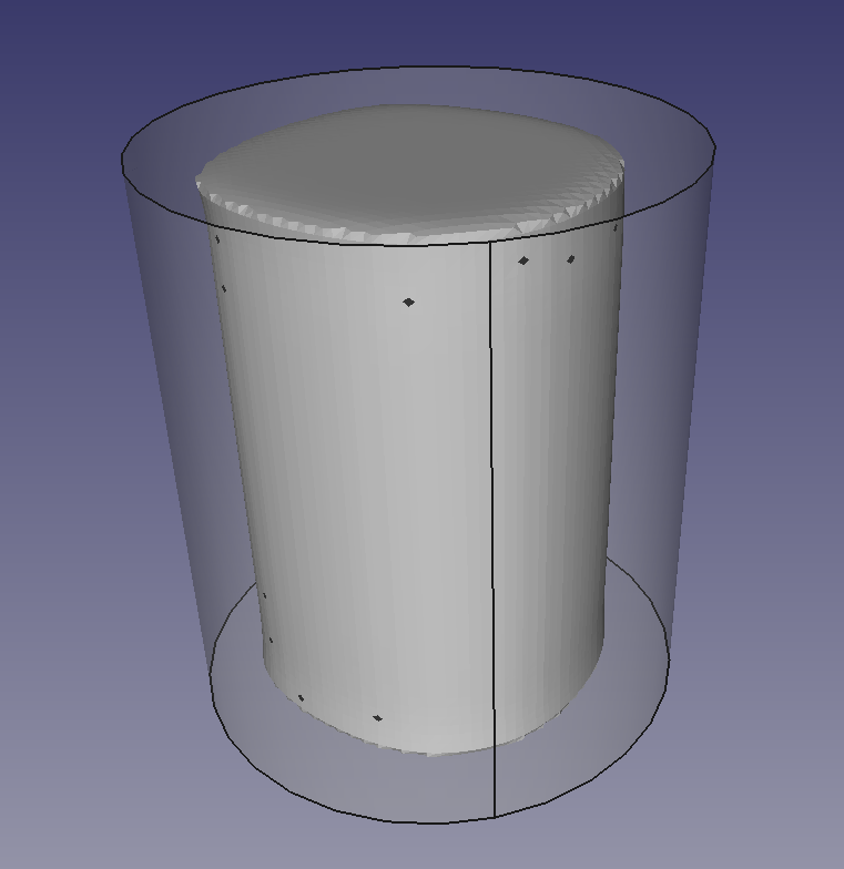
It’s printed a cylinder!
Sorry for the odd flaky triangle in the image (to be fixed). Converting the accumulated charges to a 3D model relies on Dominik Wodniok’s implementation of Marching Cubes for it’s output, incidentally, so big thanks to him.
The Effect of More Voltage or Longer Accumulated Charge (13 September)
I ran a series of tests to make cylinders like the one above, increasing the voltage applied to the electrodes, which we would expect to reduce the diameter of the resulting cylinder. Here is the result:
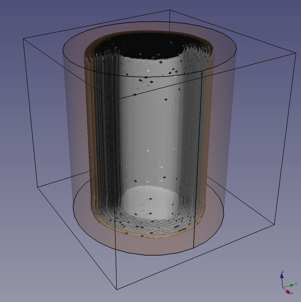
The outer box surrounds the 50x50x50 node finite-difference PDE solution grid, and the transparent cylinder is the modelled tank of the machine (outside that there is no voltage, no current, and no 3D printing material). The tank is 44 nodes in diameter. In the middle are 20 concentric separately-printed cylinders all superimposed for comparison.
Each cylinder is printed by applying +V and -V to a pair of diametrically opposed electrodes at the bottom then rotating that pattern round the bottom disc. The same thing is done for each disc upwards 50 times until the top is reached. The accumulated charge at each node from doing all that is calculated and then subjected to the sigmoid function (see the 10 August log above). The result is one printed cylinder.
That was done 20 times, increasing the value of V from 1 to 20.
All the units are arbitrary, of course; Laplace’s equation doesn’t know anything about the difference between 1 mm and 1 cm, and 1 volt or 10 volts; as long as things were consistent, the pattern would be the same. But, for sanity, let’s say that the nodes are 1 mm apart, and that when V = 1 that is 1 volt. We can then plot the radii of the resulting cylinders against applied voltage, V:
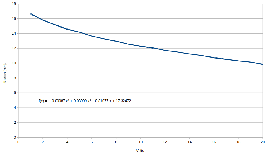
The result is not linear, unsurprisingly. But equally it is not all over the place, implying there will be a smooth radius reduction with increasing voltage. The cubic equation on the graph is a best fit (the thin, barely visible, line on the graph). There is no physical reason to expect a cubic (or any other polynomial) relationship between radius and voltage; I just wanted an empirical equation that could be used for prediction over the experimental range when it comes to trying to make more complicated shapes.
The title of this log entry says “More Voltage or Longer Accumulated Charge”. As with length and voltage, time units are arbitrary. But imagine that +/-1 volt is applied to each pair of electrodes for 1 second before stepping on. The result of doing that should be the same as applying +/-0.1 volts for 10 seconds at each pair. This is because the process is assumed to convert solid to liquid dependent on the integrated charge that each node in the grid sees (a big assumption). If the material is ohmic (another big assumption) and its resistance doesn’t change when its phase changes (a further big assumption), then this will be the case.
Finally in this log entry, a word about data processing. The result of solving the PDE is a tensor of accumulated charges at each node. These are put through the sigmoid function to see if they will be solid or liquid (or some sort of sticky half-way state), which results in another tensor of values: 1 for solid, 0 for liquid, and fractions for sticky-in-between. Those are written to a file. The marching cubes algorithm is then run over that tensor of values to create a triangulation of the imagined solid surface. That triangulation is written out as an STL file, which can then be loaded into FreeCAD and displayed, as above. With a little triangulation repair we could even print it on a conventional RepRap…
Our version of marching cubes is here on Github, and the C++ code for solving the PDE is here (along with a lot of the experimental data presented in this log).
First attempt to print a controlled shape (8 October2019)
We now have a Github repository for all the work on this project here.
If we want to print a shape, one of the things it would be useful to know is the inverse of the graph immediately above. That is to say, given a radius, what voltage should we apply to achieve it? This is the inverse of the above graph together with its fitted cubic which tells us what voltage to apply to get what radius:
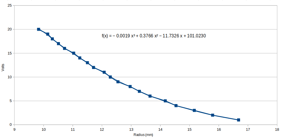
(Remember: the cubic is just an empirical fit to reproduce the curve; the coefficients have no physical significance.)
Now, as the voltages in the simulation are switched to the ring of contacts round the reaction vessel, the voltage can be set by a very simple ray-trace calculation across an imagined shape in the middle of the vessel – a rectangular block, say. The ray-trace gives the radius, and the radius gives the voltage to apply. Here is the simulated printed result:
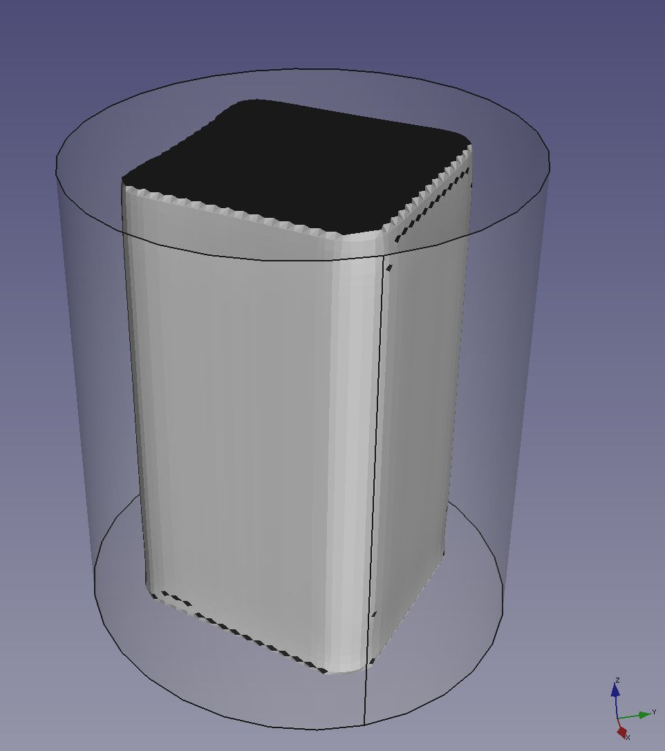
It prints, as requested, a rectangular block (the transparent cylinder is the reaction vessel, as before). The original block that was ray-traced had a square cross section 27x27x50 mm. The printed block is 25.5×25.5×50 mm. The slight reduction in size is possibly due to a cross-talk effect between higher and lower voltages, and layers influencing other layers above and below them. But the block’s faces are remarkably flat. The rounded corners are not a surprise, particularly given that the simulation only had a 50x50x50 node grid.
The block that was ray-traced then printed above was the entire height of the reaction vessel. Here is what is obtained if it is made shorter: 36mm high, placed 7mm up from the base of the reaction vessel, together with a 10mm diameter cylindrical stalk in the centre (which is rather like the support in conventional 3D printing needed to hold the object in place):
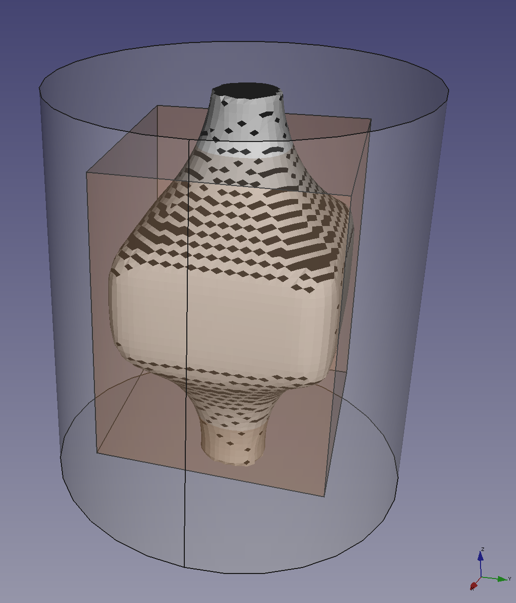
The original rectangular block that was ray-traced to create this is shown in transparent orange. As you can see, I still haven’t fixed the occasional dud triangle in the marching cubes program…
As you can also see, the effect of the high currents needed to reduce the diameter to that of the stalk top and bottom has been to erode the desired block as well. In addition, the comparitively low currents required for the rectangular block have meant that the stalk-cylinder gets fatter where it joins the block. In short, because the currents can flow freely in 3-dimensional space, there is a lot of vertical interference when trying to print in layered discs.
But, of course, with this method of 3D printing there is no need for, nor advantage to, treating the objects to be printed in layers. Any pattern of voltages can be applied anywhere over the surface of the cylindrical reaction vessel, and I have not tried using that extra freedom at all yet.
I think that will be the next step.
References and Bibliography
B. E. Kelly et al., Volumetric additive manufacturing via tomographic reconstruction, Science 10.1126/science.aau7114 (2019)
Spectra Scanner Documentation https://openeit.github.io/docs/html/index.html
Jianfeng Ping et al., Adhesive curing through low-voltage activation, Nature Communications volume 6, Article number: 8050 (2015)
To receive our newsletter which will include updates on the Electric 3D Printer click here to sign up.