Part 1 of this sequence of blog posts is here. This post assumes that you have read that one first.
Summary (TL;DR)
We made a photochromic neuron, but it suffered from a problem: the photochromic material was not fully reversible, leading to bias and drift in the characteristics of the neuron.
So we made a pure optronic neuron with four inputs. This successfully learned to distinguish simple patterns, the experimental results of which are given below.
The next stage (3rd Post, yet to be written) will be to combine many of these into an entire network and to teach that to do more complicated pattern recognition.
The Photochromic Neuron
Having made a successful optical synapse, the next stage was to go on to make an entire neuron. Here is half of it:
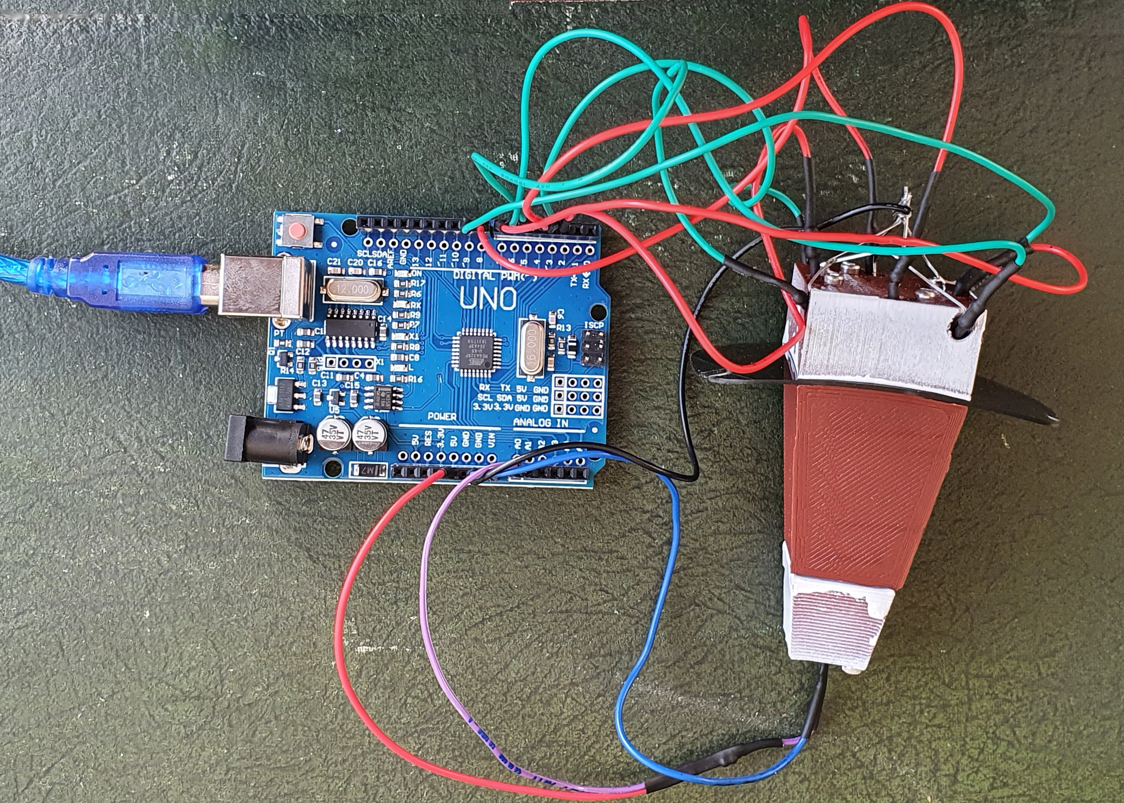
It’s controlled and monitored by an Arduino Uno. There are four visible red LEDs and four UV LEDs in the block at the top. The UV LEDs control the transmissivity of a photochromic sheet, which you can see clamped between the top block and the one below it. The red LEDs shine through the sheet to four light fibres running through the middle block that gather all the red light together and shine it on a single phototransistor in the bottom block. Here is the CAD model…
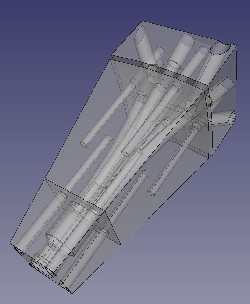
…and a diagram, in which it is easier to see what is going on:
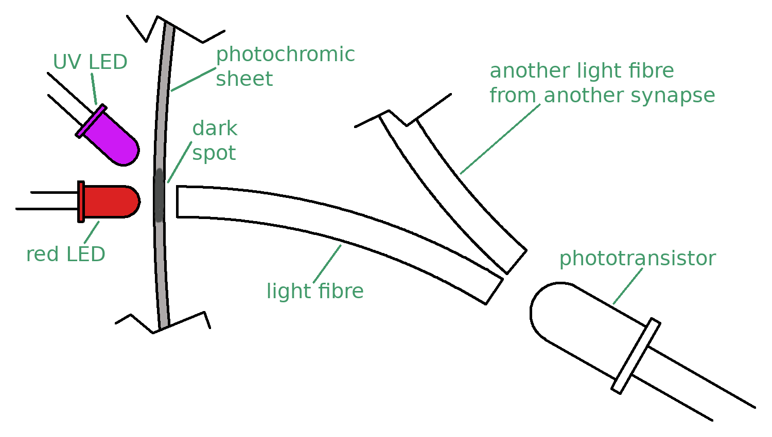
The diagram shows a single synapse, of which the neuron has four. The red LED is normally off. The UV LED is driven by a pulse-width modulated (PWM) signal from the Arduino. The mark-space ratio of the PWM signal controls how dark the spot on the photochromic sheet becomes. This continuous PWM signal keeping the spot at a certain darkness is the equivalent of memory refresh in conventional RAM, though here we effectively have an analogue memory as it can have a wide range of darknesses.
When the network is to be used the UV LED is turned off briefly, and the binary input to the synapse (1 or 0) either turns the red LED fully on, or leaves it off. The light from the LED is attenuated by the dark spot and then passes along the light fibre to the phototransistor.
There are four synapses all feeding into the one phototransistor, which adds all the light coming in in parallel, producing an output current that is proportional to the sum of all the input light.
The UV PWM signals are the inverse of the neuron’s weights, and – if the phototransistor current exceeds a threshold – the neuron fires; if not, not. When the neuron is not being used, the PWM signal is turned back on again; it is off for such a short time that the darkness of the spot doesn’t change. Similarly the red LED is on (if at all) for such a short time that it doesn’t influence the photochromic sheet, which does not respond very much to long wavelengths anyway.
As it stands, this half-neuron is a 4-input simple perceptron. There is no way that on (1) inputs (the red LEDs when on) can inhibit firing; they always make firing more likely. The other half of the neuron solves this problem, and we will introduce it below.
But first, we found a problem. When we tested this for a few hours, then left it switched off overnight. When we looked at the photochromic sheet the next morning we saw this:
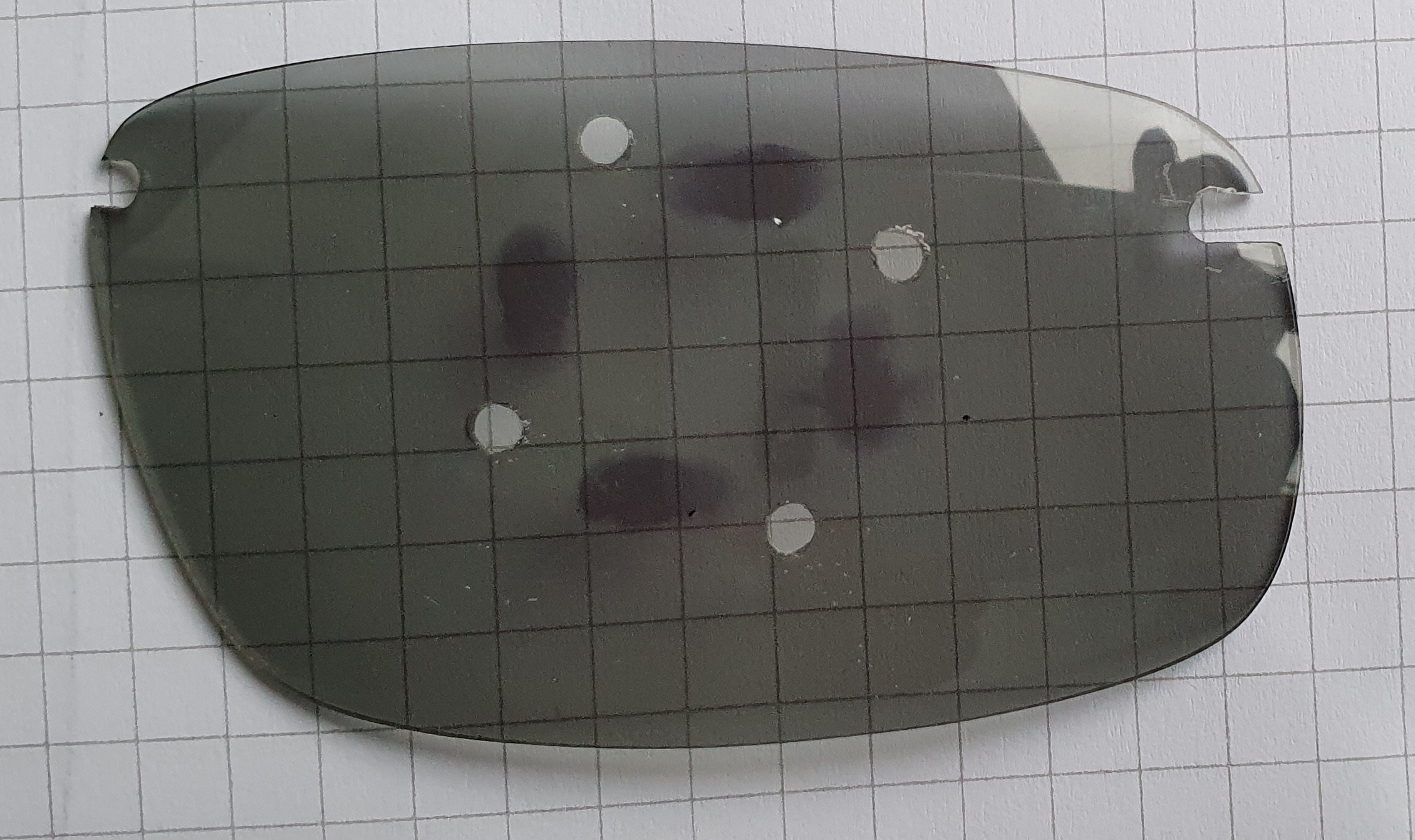
Ignore the fixing holes. The photochromic reaction is obviously not completely reversible; there are dark patches where (after about ten hours with no UV illumination) we would like to see a uniform grey across the entire sheet. This means that it is not possible to get a full range of synaptic weights using the device and, worse, the weights may well not stay constant over time when driven by a constant PWM UV signal.
The Pure Optronic Half-Neuron
Because of this we decided to abandon the photochromic approach, though we may return to it later. This is a shame, as it was the genesis of the whole idea. But a subsequent idea that was generated to solve an aspect of the photochromic system – using a single phototransistor to sum many optical synaptic inputs in parallel – can be retained. All that is needed is the ability to turn the red LEDs on and off at pre-set brightness levels, representing the weights. As before, as long as the in-use-once-taught LED on/off time is (ideally) nanoseconds, then the time taken to set the brightness (learning) can be long (remember the photochromic sheet took a minute or so to settle).
Clearly, we can’t set the LED brightness directly with a PWM signal as (unlike human eyes) a phototransistor doesn’t have persistence of vision. And even if it did, the PWM characteristics would slow the read cycle of the neural net down, when we want nanoseconds.
We designed the following LED driver circuit:
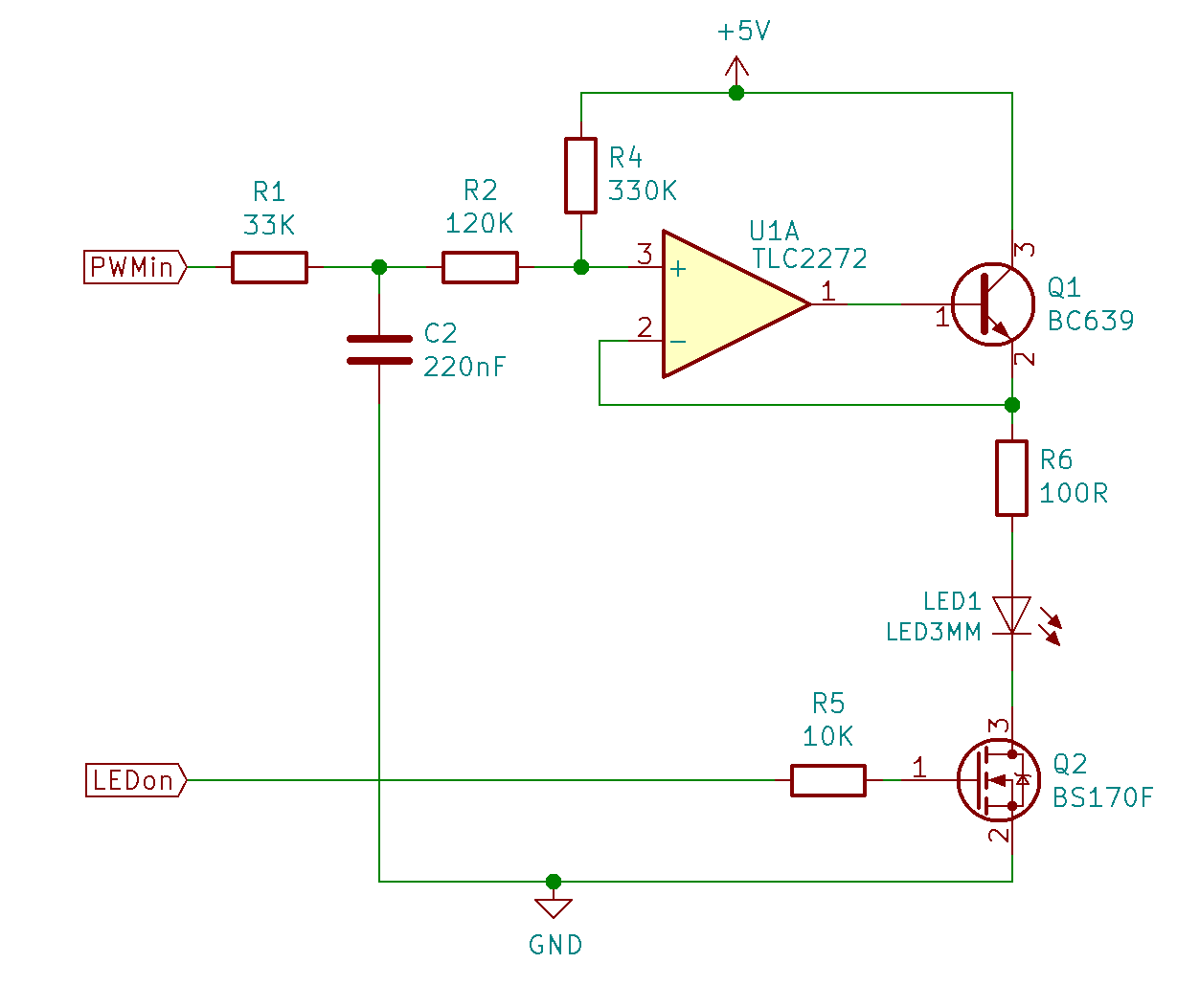
[PWMin] is a PWM signal from an Arduino at around 30KHz. R1 and C2 form a low-pass filter that converts this to a DC voltage that is buffered by the op amp U1A. R2 and R4 bias the output so that at the low end it is roughly the voltage at which LED1 turns on (about 2V), and the high end it is as near to 5V as possible. The op amp can’t supply enough current to drive the LED directly, so Q1 acts as an emitter follower to provide the 30mA that the LED needs. The voltage into the LED via the ballast resistor R6 is stabilised using the negative feedback loop of the op amp. [LEDon] causes Q2 to turn the LED on or off fast.
The voltage defined by the PWM signal and the low-pass filter takes a few tens of milliseconds to stabilise, but – as noted before – that time is not important; it represents the write cycle of the synapse weight. It is reading that has to be fast.
We made four prototypes of these LED drivers on stripboard:
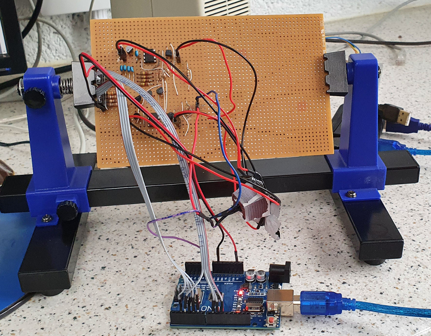
The LEDs and the phototransistor that sums their brightnesses (weights) are in the 3D-printed brown block with white paint dribbles dangling on the wires in the middle of the picture. The LEDs are under black duct tape, duct tape being an essential component of all research projects.
As mentioned above this half-neuron is just a single perceptron with no inhibitory inputs and no hidden layer. But it should be possible to teach it very simple patterns. We decided to try to get it to learn the difference between odd and even numbers, which is to say to learn just to switch on the least significant input bit and ignore the others. We taught it very crudely by repeatedly setting random PWM values for the four LEDs, allowing the low pass filters to stabilise for 300 milliseconds, then testing to see if the binary numbers from 0 to 15 were correctly classified. The network loss function was the sum of the squares of the difference between the phototransistor output voltage and a threshold value (4V) for all the wrongly classified numbers in the [0, 15] range.
Here is the output as it jumps about at random in its four-dimensional search space. Each time it finds a better PWM pattern (lower loss) than the last best it records it. The PWM values are in [0, 255].
Number of points in the search space: 20
Exploring step 1/20. Current loss: 7.64 is an improvement. PWMs: 0, 0, 0, 0
Exploring step 2/20. Current loss: 73.59
Exploring step 3/20. Current loss: 78.09
.
.
.
Exploring step 7/20. Current loss: 0.01 is an improvement. PWMs: 47, 17, 45, 5
Exploring step 8/20. Current loss: 67.66
.
.
Exploring step 19/20. Current loss: 45.26
.
Number of points in the search space: 100
Exploring step 1/100. Current loss: 0.01 is an improvement. PWMs: 47, 17, 45, 5
Exploring step 2/100. Current loss: 67.49
Exploring step 3/100. Current loss: 76.25
.
.
Exploring step 54/100. Current loss: 74.14
Exploring step 55/100. Current loss: 0.00 is an improvement. PWMs: 50, 19, 1, 9
.
.
Exploring finished.
Setting the best result: 50, 19, 1, 9,  lowest loss: 0.00

Running odd/even test:
0 is even. dv = 1.00
1 is odd. dv = -1.61
2 is even. dv = 0.68
3 is odd. dv = -1.88
4 is even. dv = 1.00
5 is odd. dv = -1.56
6 is even. dv = 0.67
7 is odd. dv = -2.01
8 is even. dv = 1.00
9 is odd. dv = -1.69
10 is even. dv = 0.63
11 is odd. dv = -2.05
12 is even. dv = 1.00
13 is odd. dv = -1.60
14 is even. dv = 0.62
15 is odd. dv = -2.17
Loss: 0.00
The dv values are the difference between the phototransistor voltage and the threshold; positive means the input binary number is even, negative means odd. The neuron learned to be a perfect classifier after 75 (= 20 + 55) jumps.
[The software (see the Github link below) also contains a Newton-Raphson loss optimiser for use in the future, but that wasn’t used for this experiment.]
Discussion and Where Next?
The device clearly works. Being made from discrete components, it is clunky. But integrated on silicon the individual synapses would be very small indeed.
And the idea of using a phototransistor to sum the inputs is very highly extensible. The smallest available subwavelength light fibres at the time of writing are about 100nm in diameter, so more than 10,000 could be fed into an area 10 microns square with hexagonal packing. In other words, it would be possible to construct a single-phototransistor half-neuron with 10,000 inputs, which is about the same as the number of inputs to a real neuron in the human brain.
It must be acknowledged that it might also be possible to feed 10,000 voltages into a summing op amp:
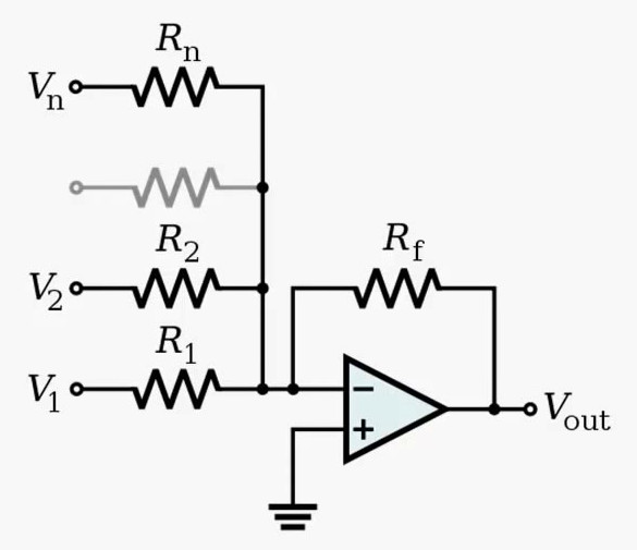
But we suspect that this would not be as fast as an optical system, and that the inputs would be more difficult to switch quickly. Also, using light allows the possibility in the future of replacing electronic parts of the device with more optical devices, which would certainly increase speed.
However, before we do all that we need to add inhibitory inputs and hidden layers to our small optronic neural network to test it further. The four-input device described above is half a neuron. The other half will be identical, and the outputs of their two phototransistors will be fed into a comparator to subtract them from each other. This will make an eight-input neuron where half the inputs are inhibitory and half exitatory. (As mentioned in the first post, that could be done by simply wiring the two phototransistors themselves as a long-tailed pair, but the comparator will be simpler to build, though less compact, initially.)
We will then arrange a number of these eight-input neurons into a network with inputs, a hidden layer, and outputs and start teaching it to distinguish more complicated patterns derived from a simple vision system.
Resources
All the files for this project can be found in our Github repository here.
Connect with us
Keep up to date on the latest RepRap Ltd news: